01 / INTERIOR STRUCTURE
Describe what lies beyond the boundary.
Explore an interior field description while retaining established Schwarzschild and Kerr solutions as local relativistic reference points.

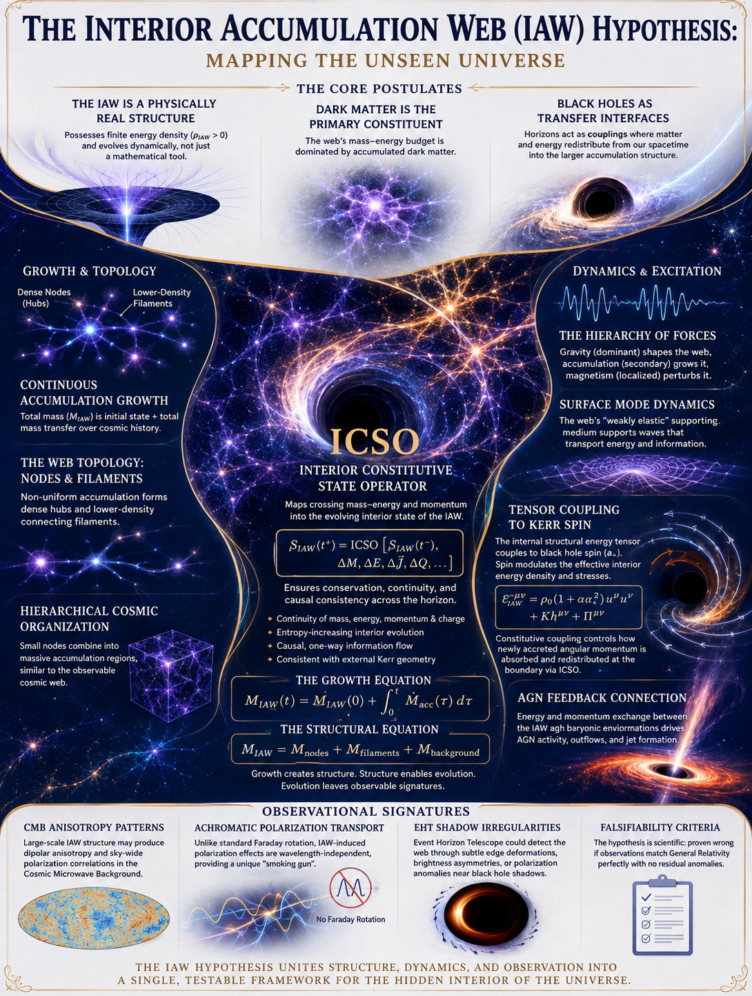
What happens inside a black hole—and how could its interior structure influence the universe beyond it?
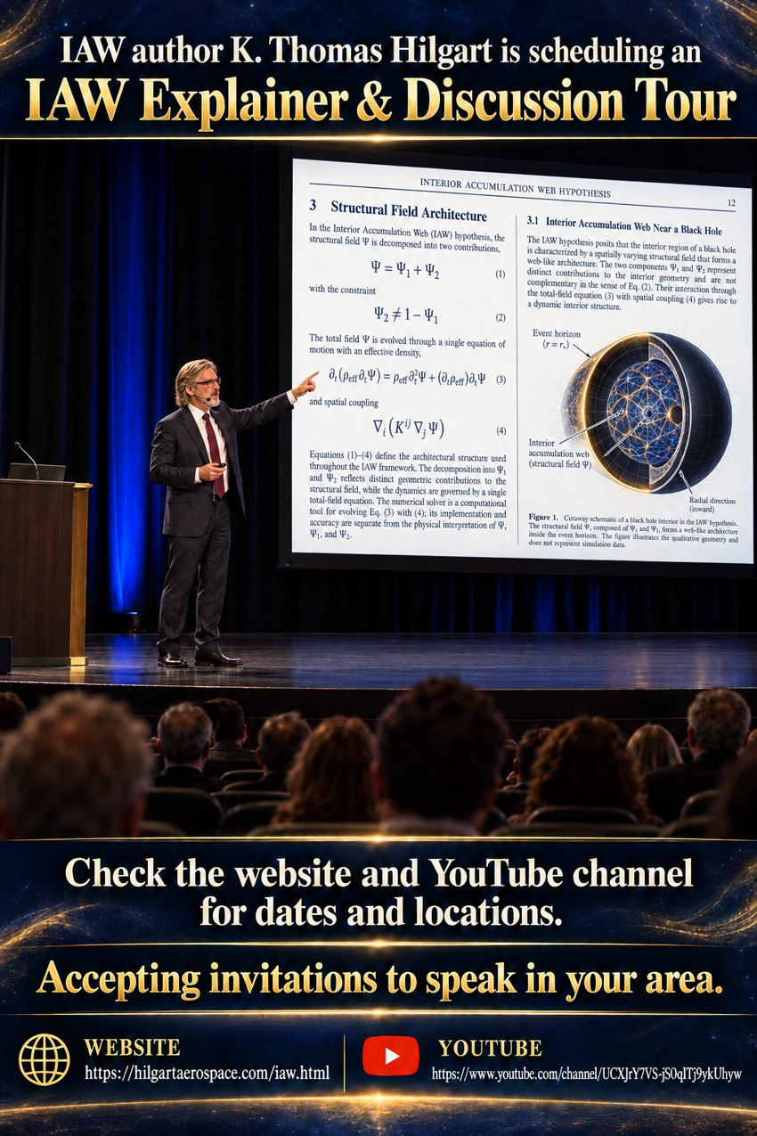
The Interior Accumulation Web (IAW) Hypothesis investigates a continuum description of black-hole interiors beyond the conditions supported by dense matter. It asks how accumulated interior structure can be described mathematically and what observable consequences could follow.
The framework begins with established relativistic gravitational physics. It explores the relationship between interior evolution, event-horizon boundaries, and larger-scale consequences, including the environments surrounding black holes.
Explore an interior field description while retaining established Schwarzschild and Kerr solutions as local relativistic reference points.
Investigate how black-hole evolution and event-horizon accumulation could relate to surrounding systems and broader cosmological behavior.
Separate proposed mechanisms from established results and identify the evidence needed to support, constrain, or reject them.

Follow the physical motivation, mathematical framework, computational work, and questions that define IAW. The manuscript is the primary reference for the hypothesis; this page provides an introduction.
Downloadable PDF
The public manuscript download will appear here when the release file is available.
Watch the IAW explanations and discussion, or listen to the introductory audio. Select a recording below to begin.
The ICSO is the computational solver used to investigate the Interior Accumulation Web. It evolves the model’s field in space and time, tracks its energy, and tests how the numerical response changes under controlled conditions.
Its development proceeded through a sequence of simulations: establish a baseline, introduce and check individual effects, audit the calculations, and reproduce the results under more demanding tests. The supplied development record culminates in Simulation 20.10, the frozen and locked solver qualification.
Follow the qualification sequence ↓PDF · 14.2 MB

The scale-invariance audit compared the same calculation under three sets of reference scales. The record retains the initial failures in 20.7 and 20.7A, followed by the corrected audit in 20.7B.
Corrections addressed the velocity comparison, the discrete gradient-energy diagnostic, and forcing-work normalization. The frozen 20.6 physics was retained; these were audit corrections, with no new physical terms.
Open original plate ↗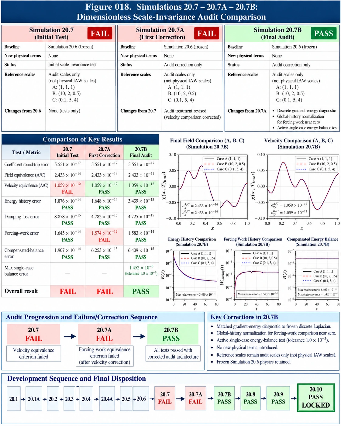
Simulation 20.9 tested seven cases: a baseline control, stronger cubic interaction, stronger linear and nonlinear damping, increased forcing amplitude, a forcing-frequency change, and combined stress.
All seven cases are marked PASS. The reported largest compensated energy-balance error was 5.87265 × 10⁻⁸, below the stated 1.0 × 10⁻⁵ acceptance limit. The plots show the different field and energy responses.
Open original plate ↗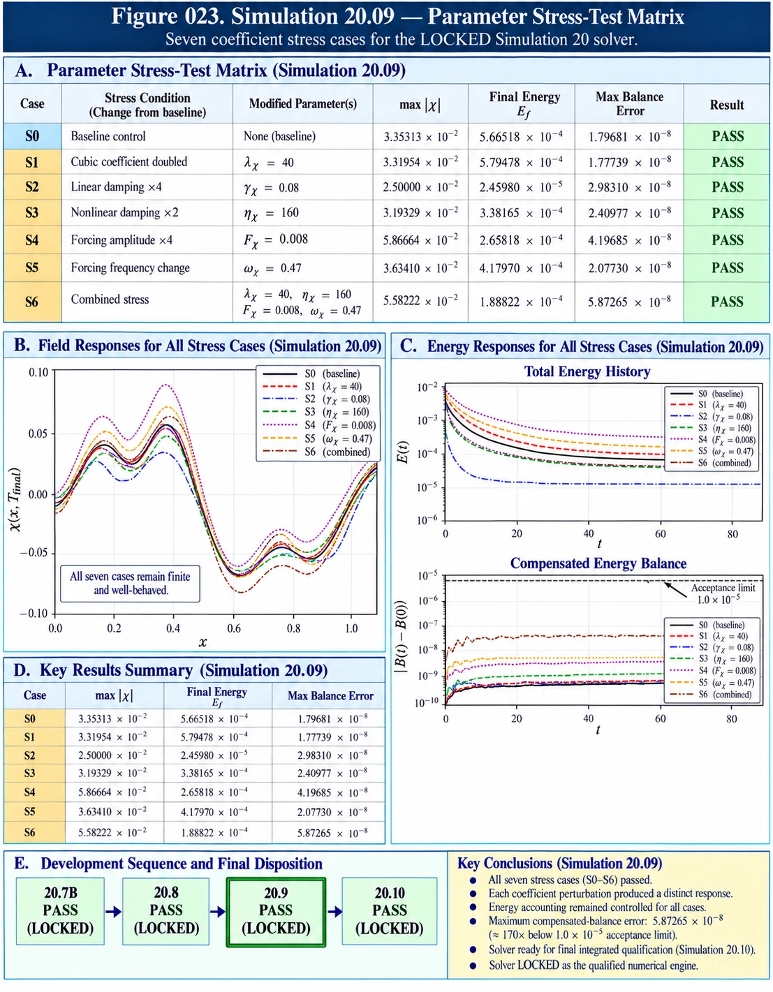
Simulation 20.10 brought the checks together: an independent baseline, the complete S0–S6 stress matrix, and an independent calculation on a finer grid. Each case is marked PASS in the supplied plate.
The baseline maximum balance error was 1.79681 × 10⁻⁸. On the 2,048-point grid it fell to 4.17965 × 10⁻⁹. The reported baseline-to-fine-grid relative field difference was 2.03063 × 10⁻³.
Open original plate ↗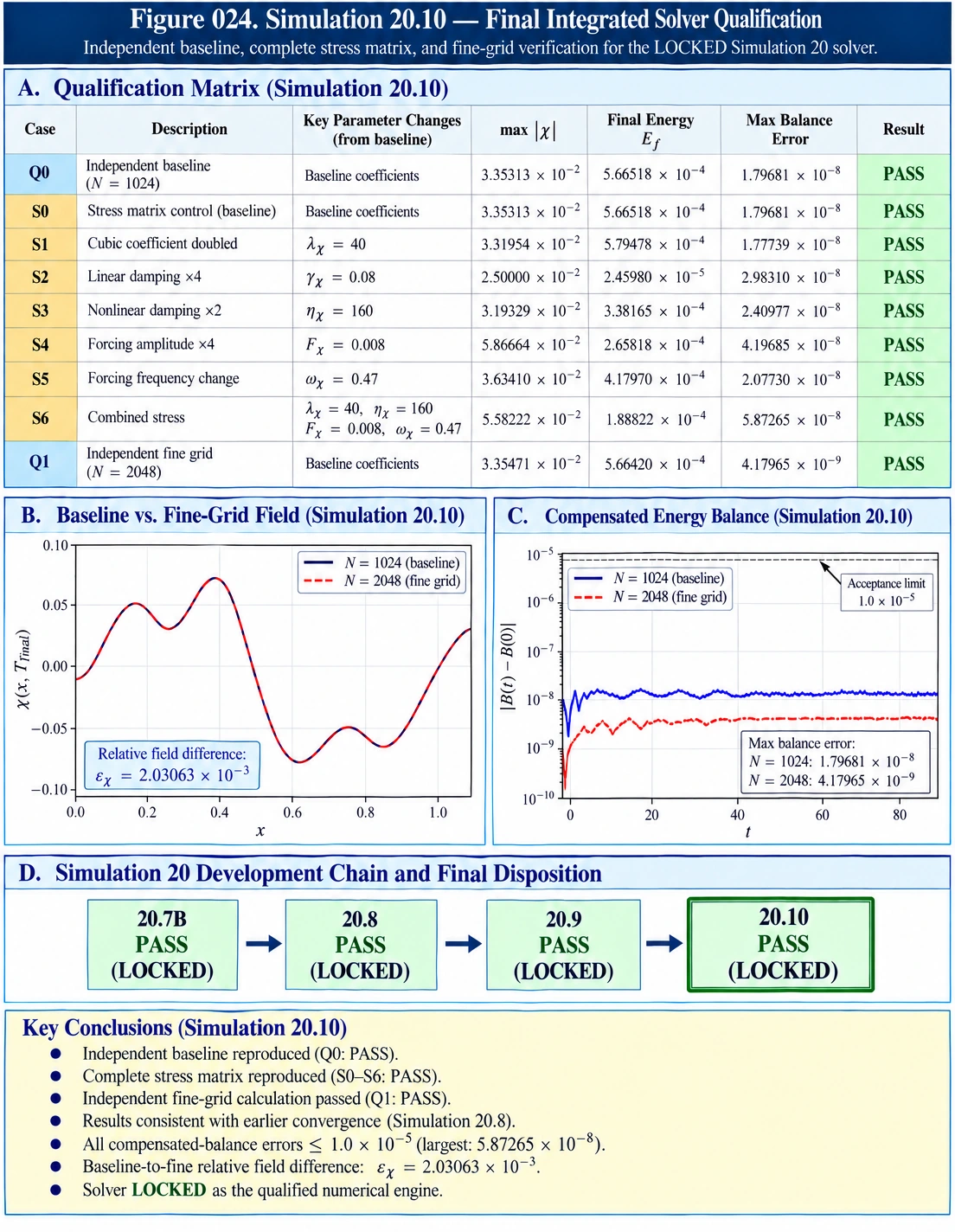
The architecture plate brings the development sequence and numerical engine onto one page: inputs, spatial operator, time integration, physics modules, stability controls, energy accounting, and output diagnostics.
Read it alongside the detailed audit and qualification plates above. These are the supplied illustrations, preserved as provided; the frozen simulation code and authoritative manuscript define the implementation.
Open original plate ↗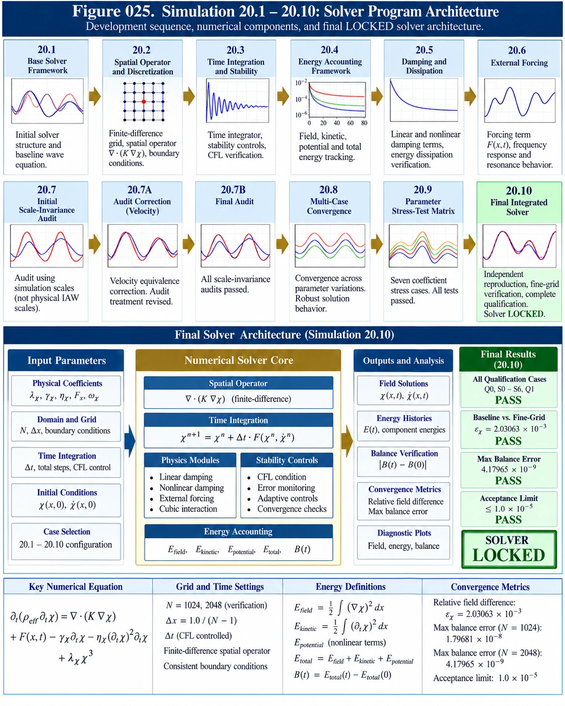
What this qualification establishes. These tests document numerical performance for the specified equations, parameters, grids, and audit procedures. They qualify the solver as a computational engine. Physical predictions of IAW are evaluated separately against observations and experiments.
IAW’s research workflow distinguishes the mathematical architecture, numerical behavior, and physical interpretation. Each addresses a different question.
Examine definitions, conservation relationships, boundary assumptions, and the consistency of the governing formulation.
Evaluate solver behavior using convergence, balance checks, and controlled parameter studies.
Identify which conclusions follow from the model and which require additional constitutive assumptions or evidence.
Develop discriminating tests and invite informed analysis of the framework, its limits, and its consequences.